Show text entries in the value area section of a Pivot Table after meeting certain conditions

In the value area section of a normal Pivot Table one can only show the result of aggregation functions such as SUM(), COUNT(), AVERAGE() etc.  Even if one drags a text field to the value area section of a Pivot Table, one cannot show those text fields because they automatically get counted.

Consider the following dataset.  The important columns to consider here are COD (Column C), Level (Column E) and Date (column G).

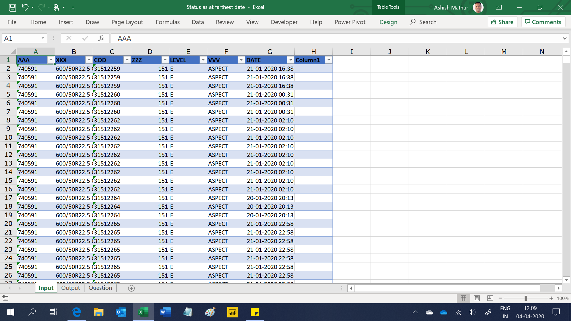
For a COD, there can be a number of rows (COD 31512268 has 3 rows).  For this COD, there is just one level (E) for the same date/time.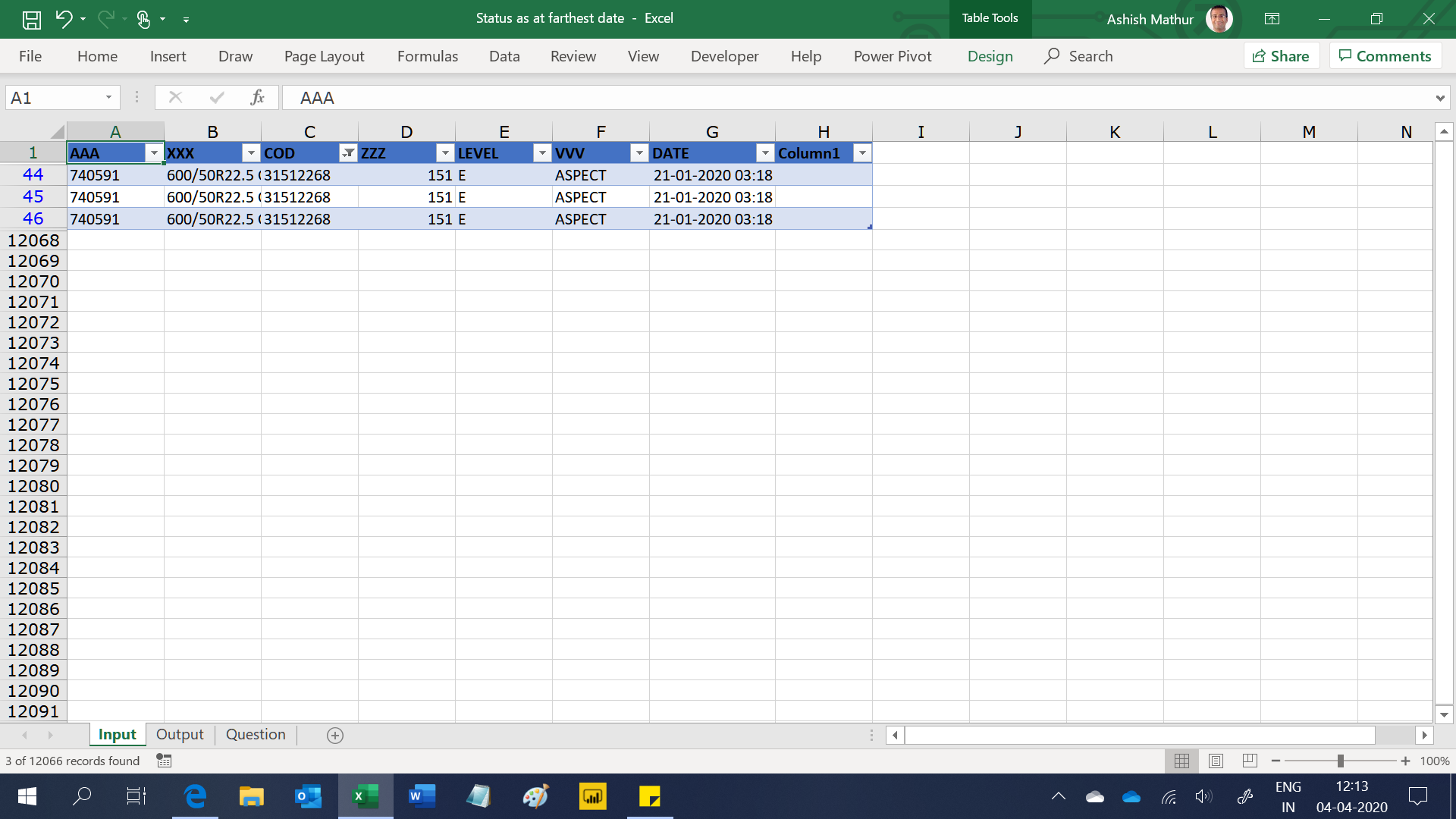
It is also possible that for a particular COD, there can be different Levels (COD 31512259 has 4 rows).  For this COD, there are 2 levels (E and D) for the same data/time.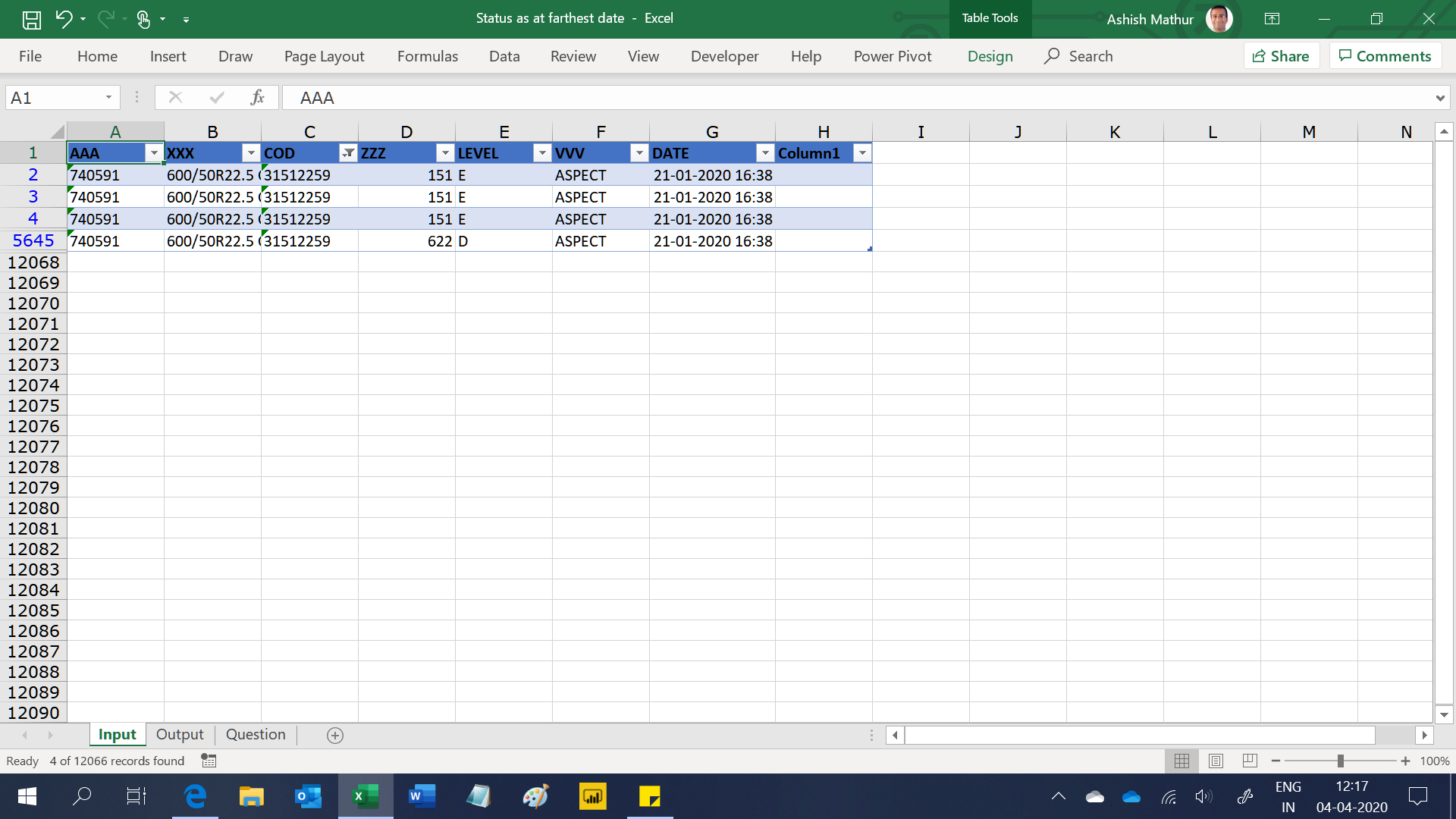

To further complicate the issue, there can be some cases where for the same date/time, a COD may have different levels.  COD 11058698 has 2 different levels (K and M) for the same date/time.
The expected result is to show a Pivot Table with COD’s in the row labels and the Level(s) as on the farthest date/time of each COD.  If a particular COD has 2 levels as on the farthest date/time, then they should be shown in the value area section of the Pivot Table (separated by commas).  So the expected result should look like this.  Notice that COD 11058698 has 2 levels as on the farthest date/time (K and M) and COD 11058700 has 3 levels as on the farthest date/time (Blank, M and 1M).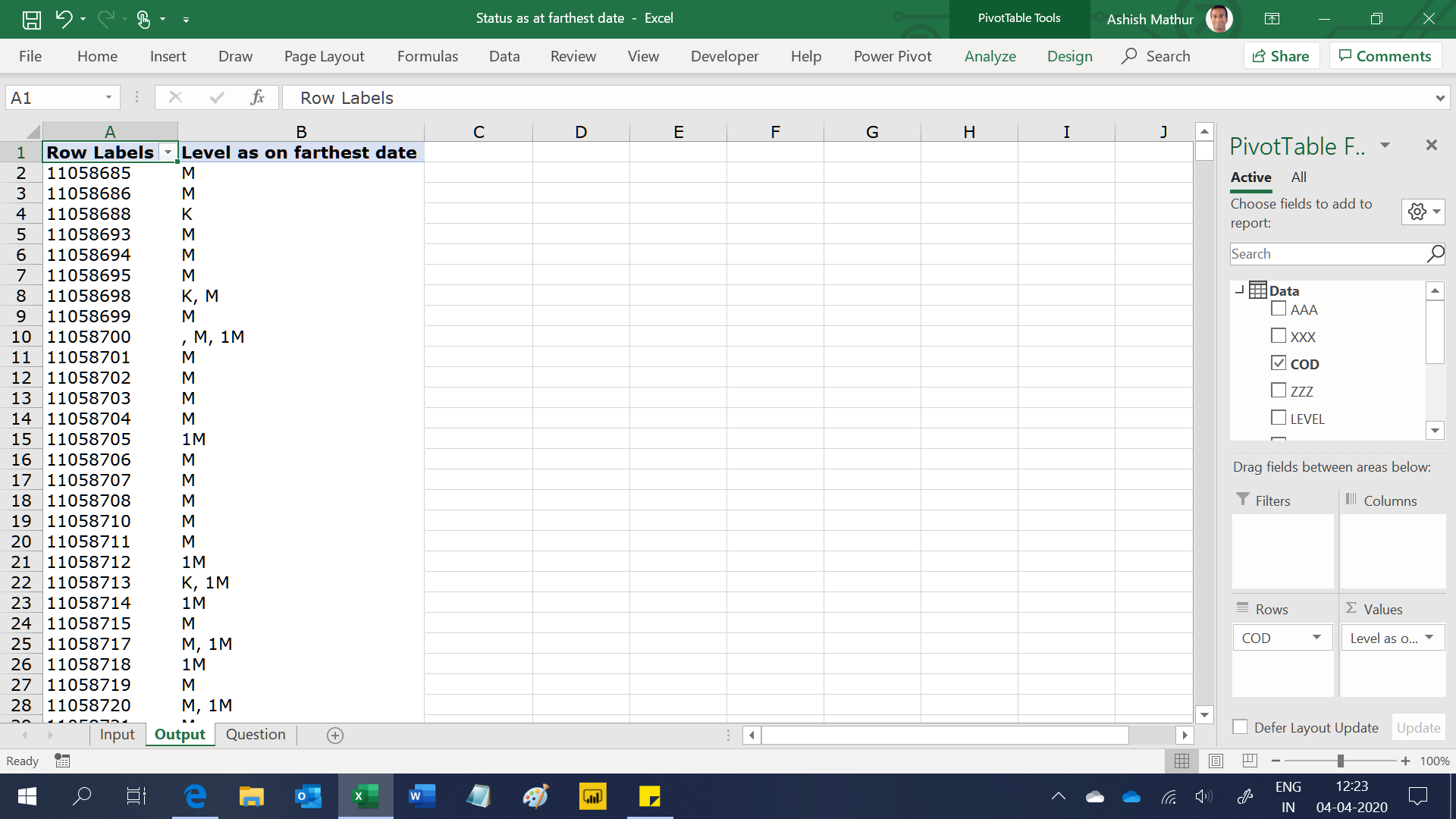
I have solved this question in MS Excel and PowerBI Desktop with the help of the DAX formulas.  You may download my Excel solution workbook from here and PowerBI Desktop file from here.