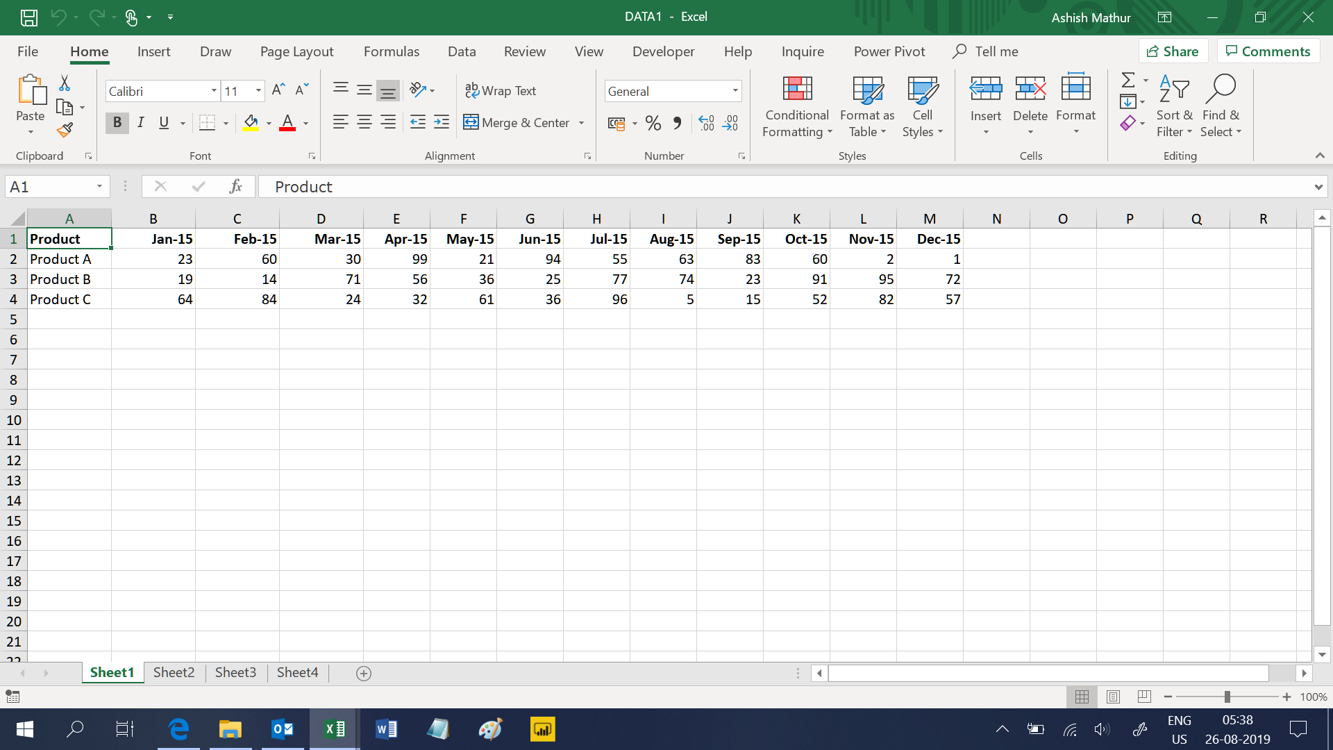
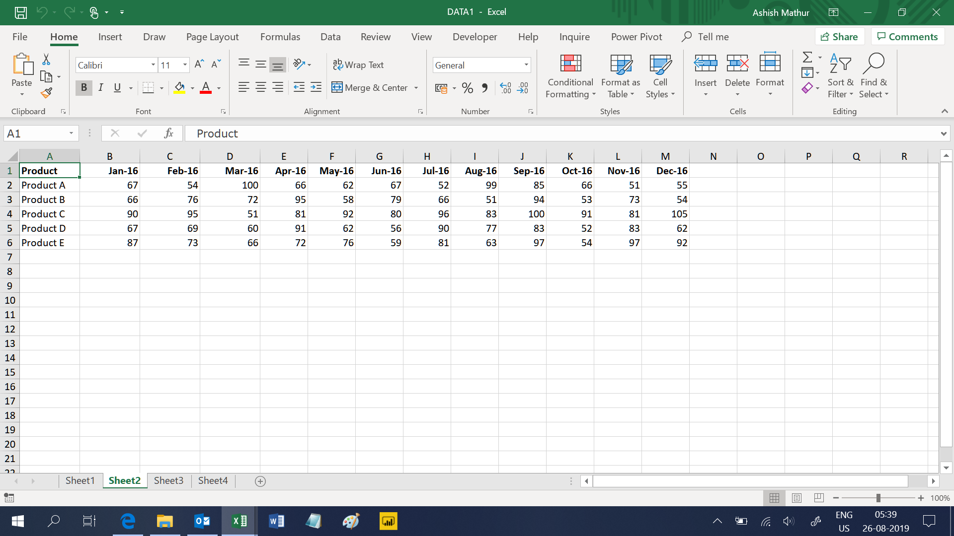
In a folder there are multiple workbooks with an unknown number of worksheets in each workbook. Each worksheet has data for one year and has 13 columns – the first is for the Product and the other 12 are for each month of the year. So sheet1 of Book1 has Product in column1, 1 Jan 2015 in column2, 1 Feb 2015 in column3 and so on until 1 Dec 2015 in column13. Likewise, sheet2 of Book1 has Product in column1, 1 Jan 2016 in column2, 1 Feb 2016 in column3 and so on until 1 Dec 2016 in column13. The worksheet which has data for the current year will have fewer columns since data for all months is not available. The number of rows on each worksheet vary depending upon the number of products sold in that year (as can be seen in the two images below).
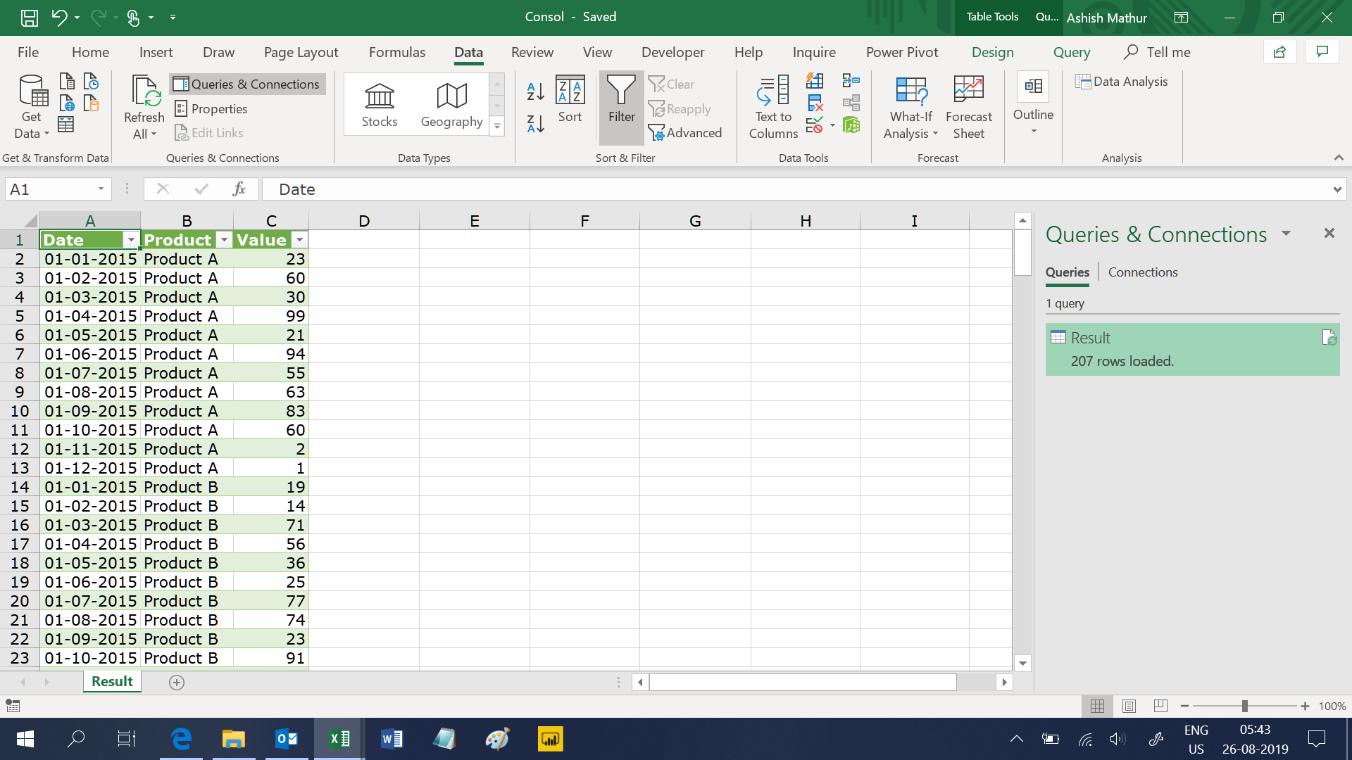
The objective is to append data from all worksheet of all workbooks to create a simple 3 column Table – Date in column1, Product in column2 and Value in column3.
The solution should be dynamic enough to accommodate the following:
- More files added to/deleted from the folder
- More worksheets added to/deleted from the existing files
- Data added by rows/columns to the existing worksheets
- Heading changes in the existing worksheets i.e. in sheet1 of the DATA1 workbook (first image above), one may want to change the year appearing in the first row from 2015 to 2013
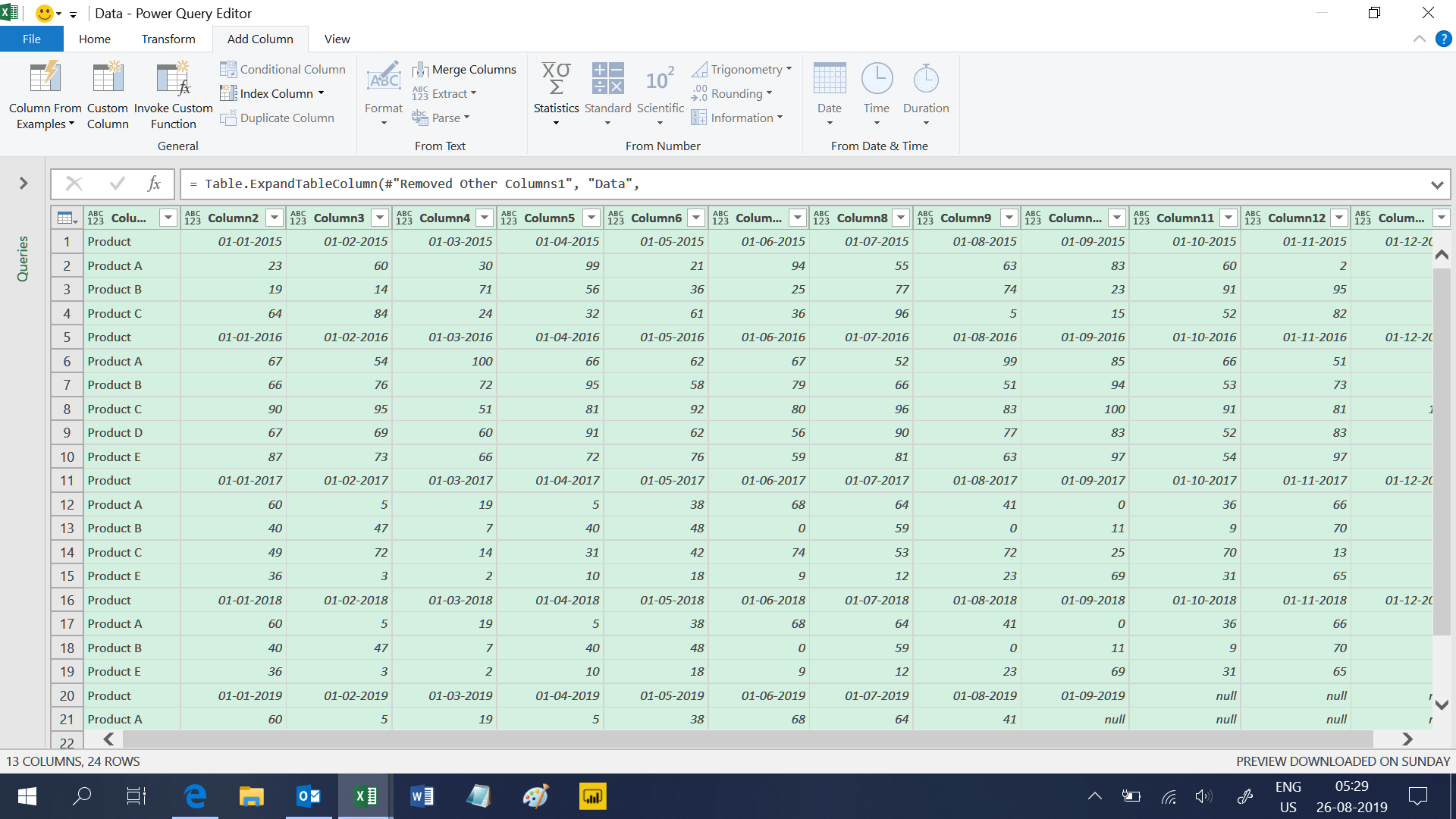
This question would have been an easy one to solve had the headings on all worksheets of all workbooks been the same such as Month1, Month2, Month3, Month4 etc. In that scenario, the technique shown in this YouTube vide would have worked very well. However, since the headers on each worksheet of each workbook are different, this technique yields an unexpected result (shown below) – Please note that I have not used the Table.PromoteHeaders([Data]) command as described in the video because that would take away the row with dates i.e. row1, row5, row11, row16. If I do not run that step, I get the output as shown in the image below. The dates appear as part of the Data rather than being identified as headers.
I have solved this question using the Power Query Editor. You may download my source data from here and solution workbook from here.
- Download the source data workbooks and save them in a folder.
- Download the solution workbook and save it anywhere else.
- Open the solution workbook and go to Data > Queries and Connections.
- In the pane that opens up, right click on the Query > Edit.
- In the Applied steps window, double click on Source and specify the path where you have saved the source data workbooks (step1 above).
- Click on OK > Close and Apply.
Append data from multiple worksheets of multiple workbooks where each worksheet has a different heading
{ 0 Comments }