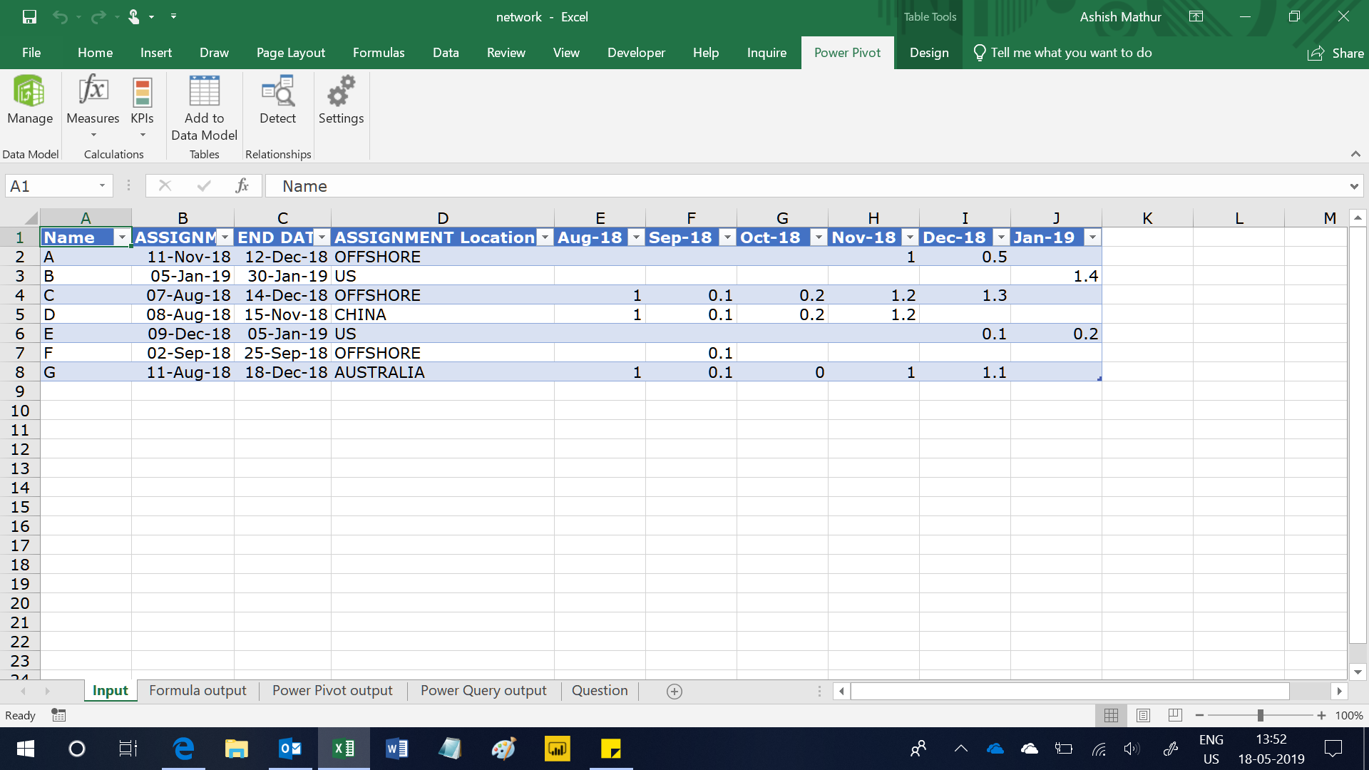
In the dataset below column A has the Employee Name, column B and C are the assignment start and end dates, Column D is the location and columns E to J are the Month-Year columns. So each row represents data for an employee on a particular project. The numbers in range E2:J8 represent how much that particular employee is aligned to the particular project i.e. a value of 1 means that the employee is dedicated solely to that project, 1.4 means that the employee will be spending extra hours on that project and 0.1 indicates that the employee will be working on multiple other projects.
The objective is to create another column (column K in the second screenshot) which will show the number of hours the employee will spend on the project. The number of hours will be computed as number of working days in a month (treat Saturday and Sunday as weekends) * time allocation to that project (the numbers in range E2:J8) * 8.5 hours per day for an Offshore project and 8 hours per day for other projects.
The raw data sheet looks like this
The expected result is
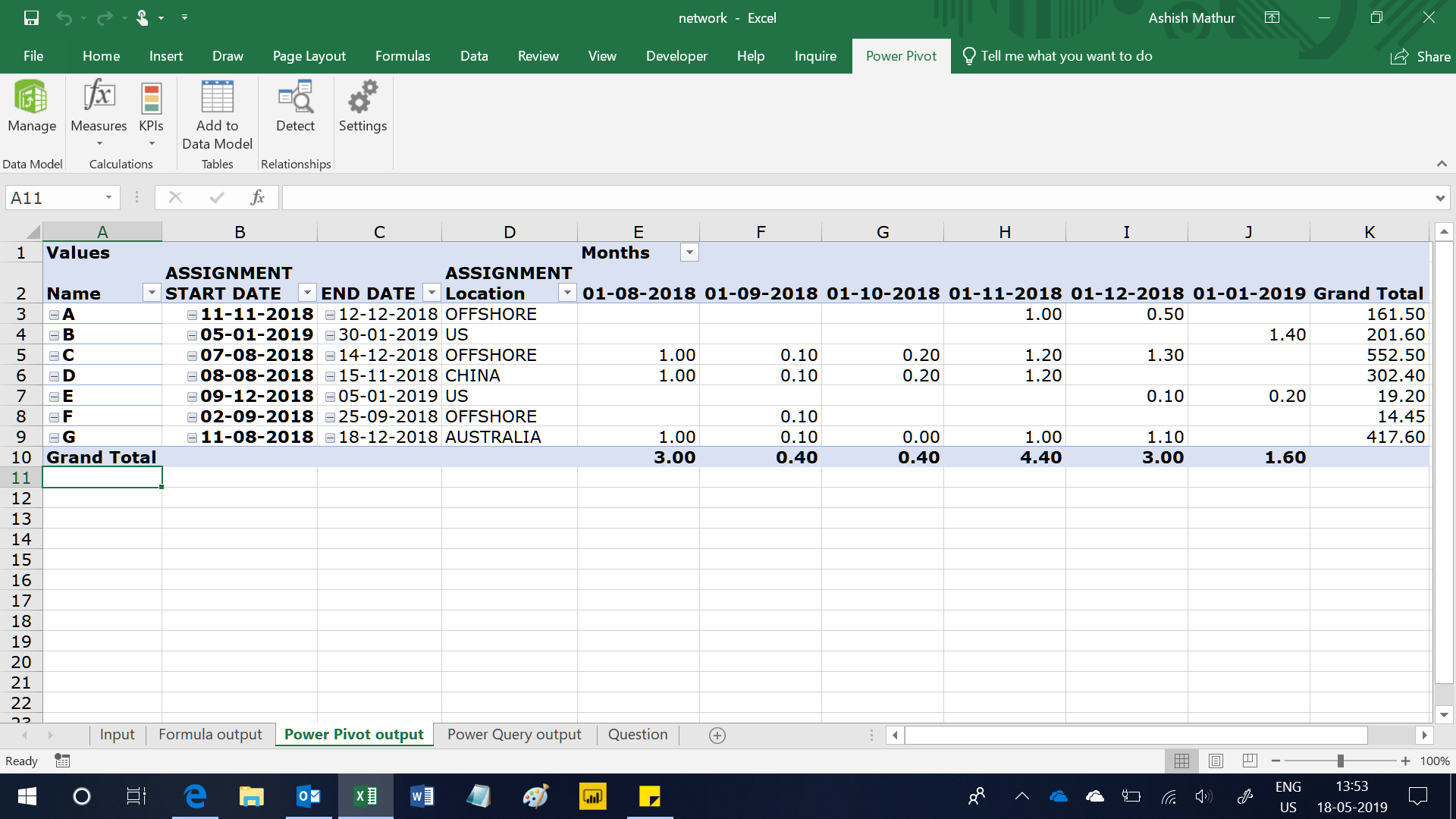
The figure in cell K3 has been computed as:
- Number of working days between November 11, 2018 and November 30, 2018 are 15. So 15 * 1 = 15
- Number of working days between December 1, 2018 and December 12, 2018 are 8. So 8 * 0.5 = 4
- Total effective working days are 15 + 4 = 19
- Since it is an Offshore project, the hours per day would be 8.5. Therefore total effective hours: 19 * 8.5 = 161.5
I have solved this problem using 3 methods:
- Excel formulas – Refer worksheet named “Formula output”
- Power Query and PowerPivot – Refer worksheet named “Power Pivot output”
- Power Query only – Refer worksheet named “Power Query output”
You may download my solution workbook from here.
2 Trackbacks