The title sounds confusing!!!!. Please bear with me and read on. Here’s a simple dataset
| Client ID | Client Name | Resource | Project ID | Billable amount |
| 1 | Alpha | David | 1000 | 10 |
| 1 | Alpha | Henry | 1001 | 20 |
| 1 | Alpha | Rakesh | 1002 | 30 |
| 1 | Alpha | Alice | 1003 | 40 |
| 2 | Beta | Alice | 1000 | 50 |
| 2 | Beta | Alicia | 1002 | 60 |
| 2 | Beta | Patrick | 1003 | 70 |
| 2 | Beta | Mukesh | 1004 | 80 |
| 2 | Beta | Suresh | 1006 | 90 |
| 2 | Beta | Ajay | 1005 | 100 |
| 3 | Gamma | Rama | 1004 | 110 |
| 3 | Gamma | Sakshi | 1006 | 120 |
| 4 | Theta | Prabhu | 1005 | 130 |
| 5 | Epsilon | Alice | 1000 | 140 |
| 5 | Epsilon | Alicia | 1001 | 150 |
| 5 | Epsilon | Prabhu | 1002 | 160 |
| 5 | Epsilon | Sakshi | 1003 | 170 |
| 5 | Epsilon | Raghav | 1008 | 180 |
| 5 | Epsilon | David | 1010 | 190 |
| 5 | Epsilon | Henry | 1012 | 200 |
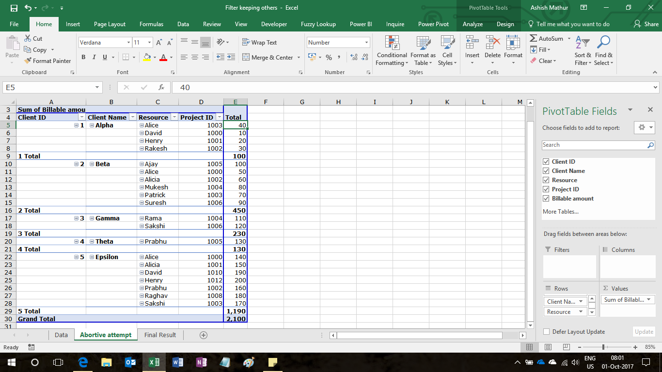
Here’s a Pivot Table built from the dataset above.
The question is “Is there a way to show only those rows of data which have Alice but also show others who worked with Alice”. While the first part of the question can be answered easily by filtering the Resource column on Alice, the second part (italicized for your reference) of the question is the real challenge. When one filters the Resource column on Alice, the result is as seen below:
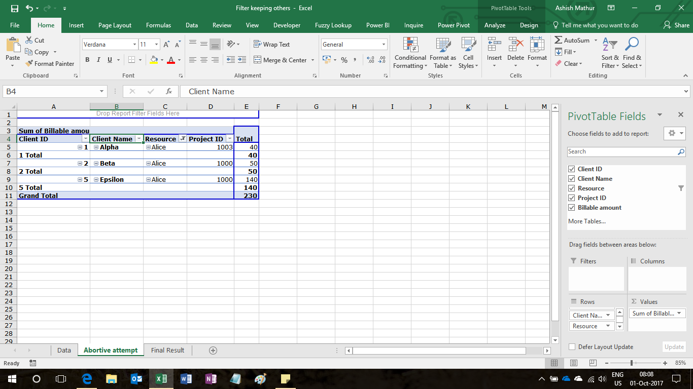
This view does not show me who else worked with Alice. The result I am expecting to see is:
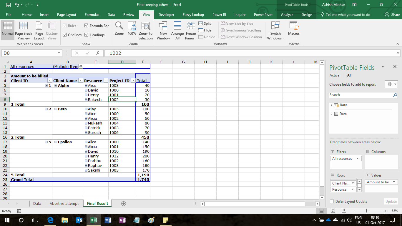
This problem can be resolved with the help of the Query Editor (Power Query). The basic idea is to create another column in the original dataset where we create a string of all resources for every row. So for example, in every row of Client ID1, the sixth column should show David,Henry,Rakesh.Alice and so on. Once this is done, one can simply take this column to the Report filter section of the Pivot Table (see last image above) and filter on Alice.
You may refer to my solution in this workbook.
2 Trackbacks