Any well arranged dataset should be “Pivot Table” ready with the following 3 important properties:
- There should be no merged and centered cells; and
- Every column should have a unique heading; and
- Every column should have only 1 heading
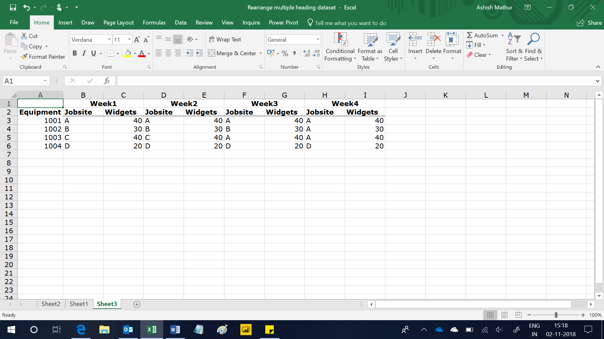
Here’s one dataset which violates all rules mentioned above.
- Headings in row 1 are merged; and
- The headings in row 2 are not unique
- Every column has headings in row 1 and row 2.
To be Pivot Table friendly, this dataset will have to be restructured into a 4 column one – Week, Equipment, Jobsite and Widgets as shown below:

I have achieved the desired result by using Data > Get & Transform (also known as Power Query in earlier versions of MS Excel). The solution is dynamic for new rows and columns added to the data on the Input worksheet – one simple has to go to Data > Refresh All. You may download my solution workbook from here.
In this workbook, there is another example of how one can transform a multi heading dataset into a Pivot Table ready dataset. The primary difference between this and the previous dataset is that there are 2 descriptive columns to the left (as against only one in the previous example).
Rearrange a multi heading dataset into a single heading one which is Pivot ready
{ 8 Comments }