Here is a simple 5 column dataset showing basic employee information.
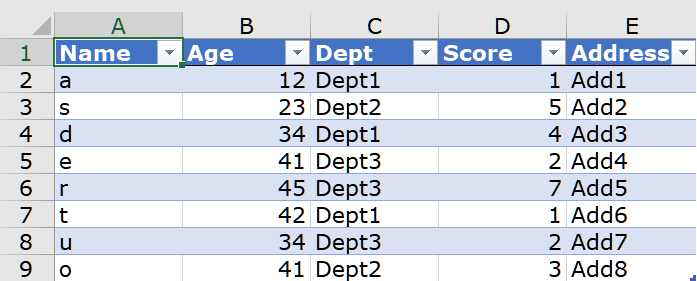
The objective is to show only those rows of data in which the Score (column D) is greater then 3. While one can solve this with a simple filter, the solution will not be dynamic. To get a dynamic solution, one may use the FILTER() dynamic array function that comes with the Microsoft 365 subscription service.
In cell G2, one may simply write this formula
=FILTER(A2:E9,D2:D9>3)
This is a far better solution because it is formula driven and thereby dynamic. So all good till here. Now let’s make it a little interesting.
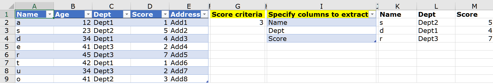
The revised objective is to show only those rows of data in which the Score (column D) is greater then 3 and only display 3 columns – Name, Department and Score (columns 1,3 and 4) in the end result. This can be solved using Data > Advanced filter but the result will be static. To get a dynamic solution, one may use a nested FILTER() function in cell G2
=FILTER(FILTER(A2:E9,D2:D9>3),{1,0,1,1,0})
This formula will return the same number of rows (3 rows) as the previous FILTER() function returned with only 3 columns – Name, Department and Score. The 1’s and 0’s in the formula denote whether one would like to see the particular column in the end result or not. So once again, all good till here.
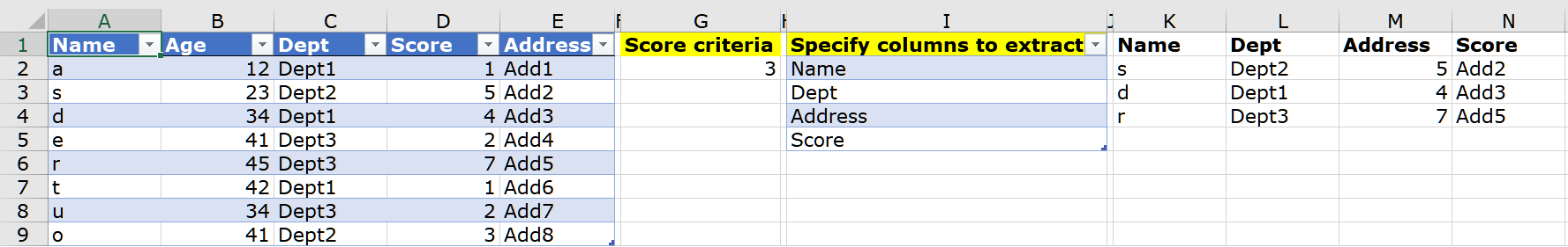
Now, let’s take it a notch higher. What is there were 35 columns in the original dataset and one wanted to see data appearing in columns 1,6,22,25,29 and 34. It will be quite time consuming to enter the 1’s and 0’s in order within the FILTER() function. So the question here is how does one save time and effort? Ideally one should be able to just enter the column headings one wants to see in the end result.
As you can observe in the image above, one has to simply specify the columns to extract in column C and the result populates from column K rightwards and downwards. Using dynamic array formulas and the FILTER() function, one saves effort in entering 1’s and 0’s in the FILTER() function (the FILTER() function has been written in cell K2 – download link of the file is shared below). If one types Address in cell I5, then Address would automatically appear in cell N1 and so will the entries in range N2:N4. So this does seem like a good solution. So while it is good, it is not a perfect solution. In column I, if one changes the order of the headings i.e. one enters Name, Dept, Address and Score (rather than Name, Dept, Score and Address), the result under columns M and N would be incorrect (see image below).
Solving this challenge led me to using Data > Get & Transform. I made use of the latest feature introduced in Power Query called “Data Types” (I received this feature update on December 4, 2020).
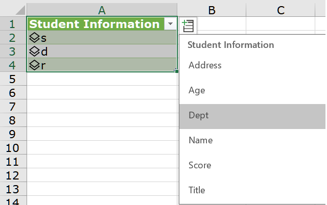
As one can see in the image above, one simply has to select any heading one wants and that appears in the next available column.
You may download my solution workbook from here in which i have shown both formula based and the Power Query solution.
2 Trackbacks